Audio Reactive Programming: Envelope Followers

My weirdly specific hobby is coding visuals that react to music. (See here or here.) I thought I would share some of my audio processing and animation tricks. Most of my techniques for synchronizing animations to music start with envelope followers. In this article, I’ll explain what an envelope follower is and how it works. In a future article, I’ll give some examples of how to use one.

Let’s take a short percussion sample and look at its waveform:

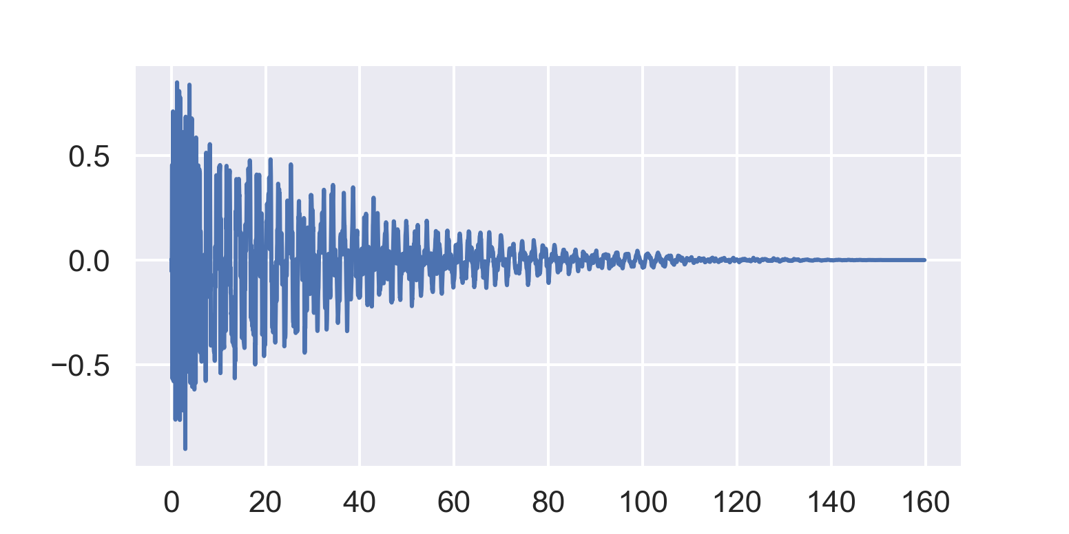
It suddenly gets loud, then slowly fades back down to zero. If you grabbed a pen and tried to trace the contour of the waveform, you might come up with something like this:

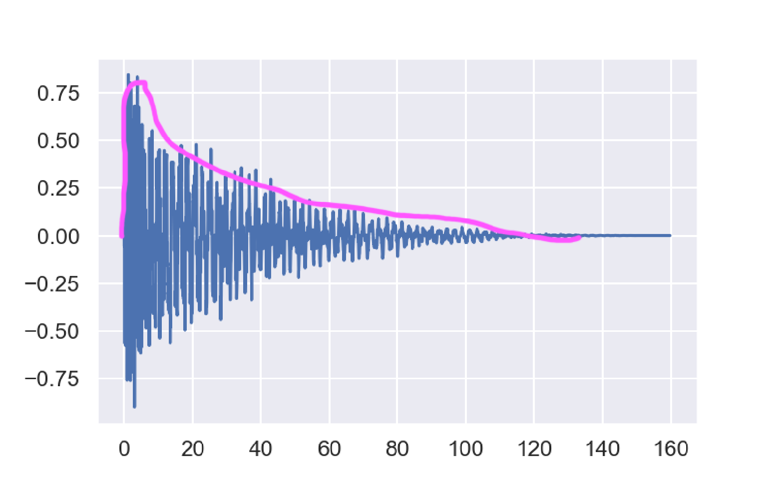
The idea of an envelope follower is to mathematically extract that contour from the raw waveform.

How would you do that?

Let’s zoom waaaaay in on the wave form:

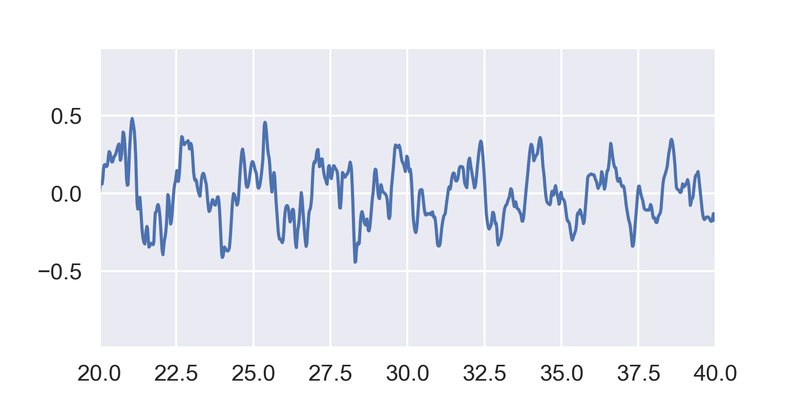
You can see that there’s an oscillating pattern that goes up and down on the scale of about 2 milliseconds. Two milliseconds is far below the time limit of human perception. You can’t hear the volume changing that fast; instead you hear a tone of around 500 Hz. If it were repeating closer to 1 ms, you’d perceive a higher-pitched tone, etc. Even though these fast level changes are present throughout the waveform, they don’t “sound” like a change in perceived volume to your ear. The changes are present in the waveform, but we want the envelope follower to ignore them.

Now let’s zoom out and repeat the whole sample back to back a few times:

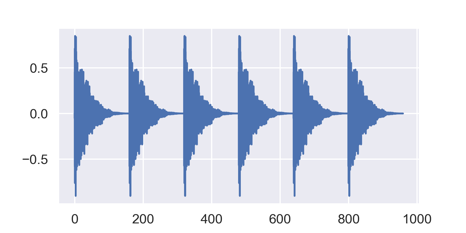
This is also a repeating pattern that goes up and down, and repeats roughly every 180 ms. But on this scale, you’ll hear it as a sequence of distinct clicks. We want our envelope follower to track these distinct clicks, while ignoring the local wiggly changes.

One idea is to just average some chunk of the waveform together. If you average over a chunk that’s longer than 2 ms, you’ll smooth out the entire repeating pattern we saw above. But remember that the waveform is negative half the time, so the raw average will generally hang out around zero. Instead, averaging the absolute value of the signal will work better:

class Follower1 {
public:
  Follower1(size_t bufsize) :
    buffer_(bufsize, 0), i_(0) {}

  double process(double x) {
    buffer_[i_] = abs(x);
    i_ = (i_ + 1) % buffer_.size();
    // pretend we have an average function
    return average(buffer);
  }

private:
  std::vector<double> buffer_;
  size_t i_;
};

At 44.1 kHz samplerate, 1 ms is just over 40 samples. So bufsize = 128 is roughly 3 ms:

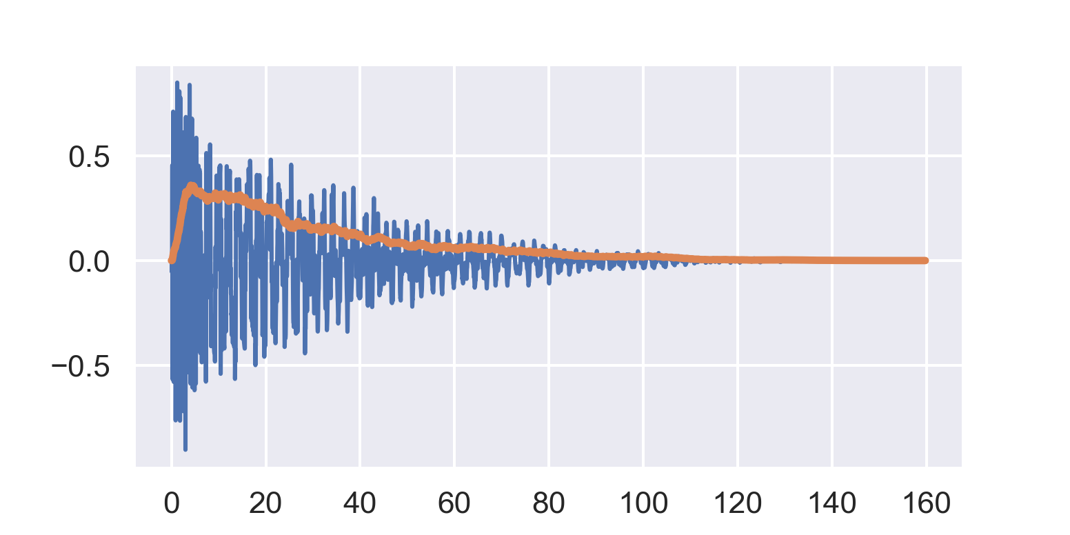
This works ok – it’s roughly following the shape of the signal. It’s a little wobbly though. Compare with bufsize = 512:

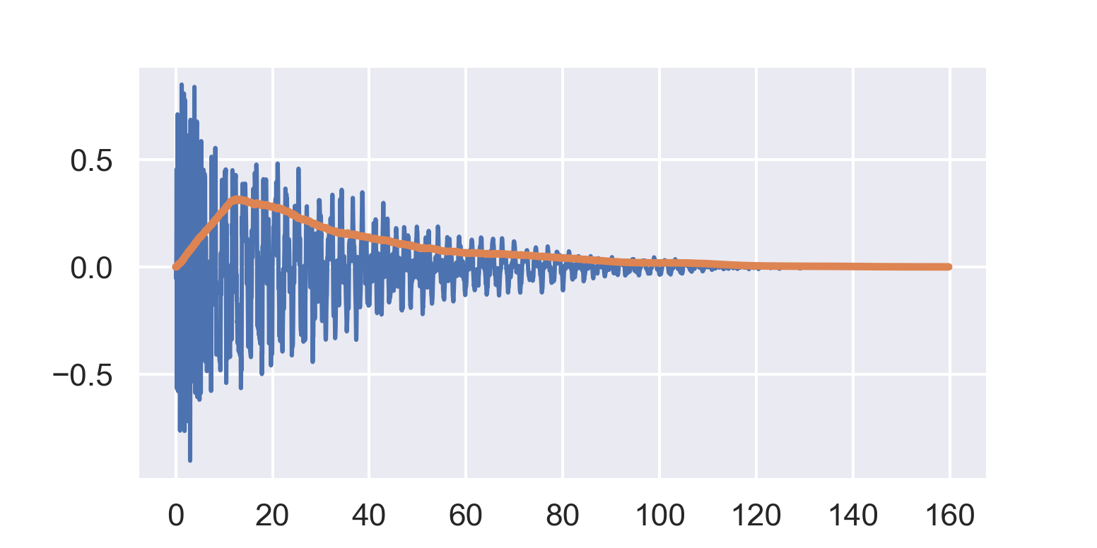
This time the buffer is around 12 ms. This envelope is smoother, but the initial peak is sort of delayed. That’s the tradeoff: short buffers are more responsive to sharp peaks, whereas long buffers produce smoother envelopes.

This kind of follower is probably adequate for many purposes. But is it really necessary to allocate that circular buffer? Nope!

We don’t need no stinking buffers

Here’s an alternate implementation that may look a little strange at first:

class Follower2 {
public:
  // a should be between 0 and 1
  Follower2(double a) :
    a_(a), y_(0) {}

  double process(double x) {
    const auto abs_x = abs(x);
    y_ = a_ * y_ + (1 - a_) * abs_x;
    return y_;
  }

private:
  double a_, y_;
};

What’s going on here? This is the key line:

y_ = a_ * y_ + (1 - a_) * abs_x;

To help us understand what’s going us, let’s drop one factor:

y_ = a_ * y_ + abs_x;

Every time we process a new value from the input, we scale the previous output by a_, add in the new value, and remember that new blended value. If you unroll this a few rounds you get a formula like:

y_ = x_0 +
     a_ * x_1 +
     a_^2 * x_2 +
     a_^3 * x_3 +
     a_^4 * x_4 + ...

where x_0 is the current input, x_1 is the previous input, x_2 is the one before that, etc.

Since a < 1, each successive power of a gets smaller. Therefore y becomes a weighted average of all the preceding input values, with older values weighted lower. If a = 0.9, the weight will be 0.9 for the previous value, 0.81 for the one before that, 0.73 for the one before that, etc. In a sense, each value of y_ contains a memory of every input value it’s seen so far.

When a is small, the successive powers of a go to zero very quickly: this means we average over a short time window. When a is closer to 1, the powers decay more slowly, and we effectively average over a longer time window.

OK, then what’s the deal with the (1 - a_) in the original code snippet? All that does is scale the entire output signal. Specifically, (1 - a_) is the scale that ensures the output envelope does not exceed the peak magnitude of the input envelope.

If we run our sample through this follower with a = 0.98, we’ll get:

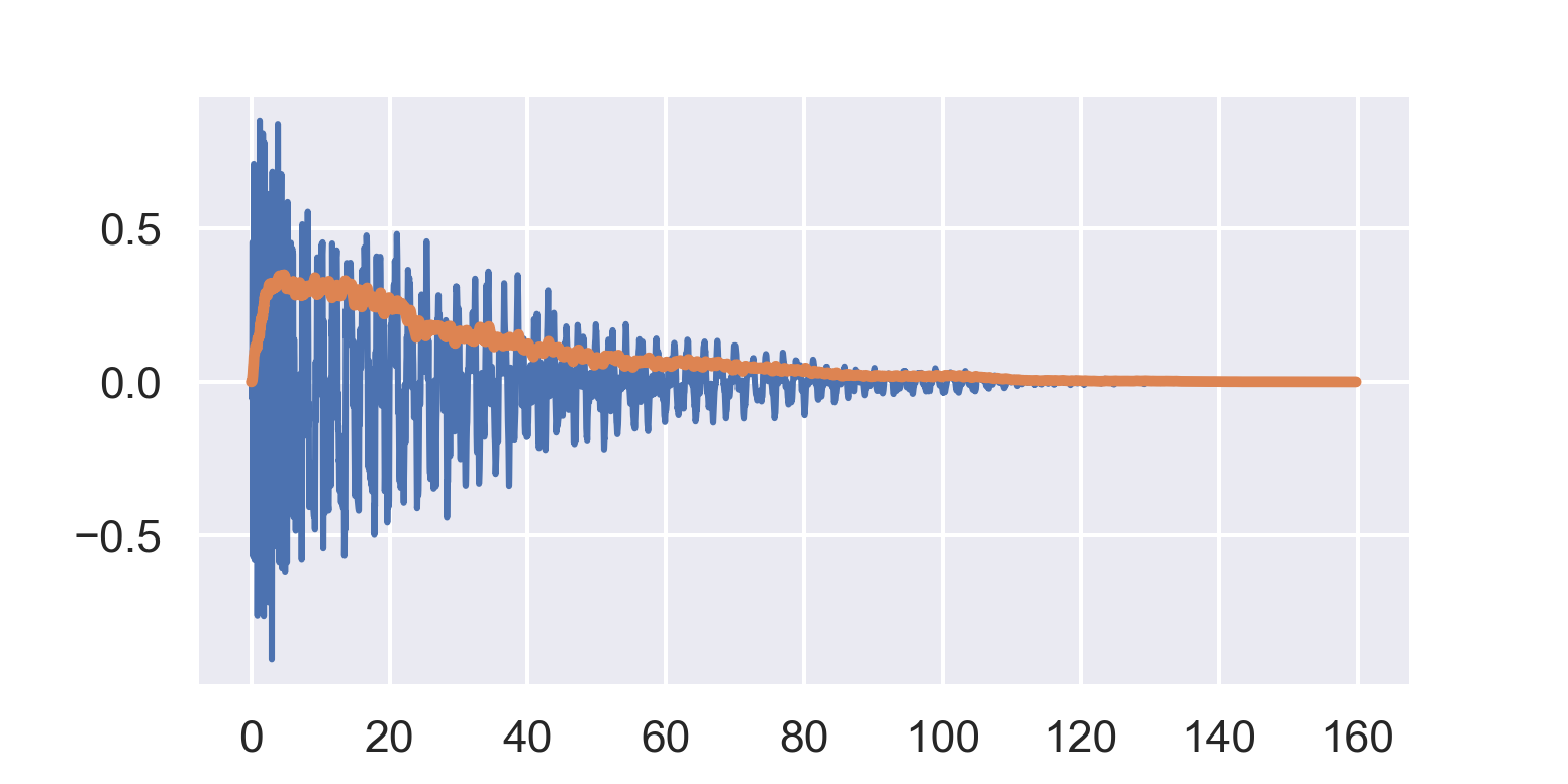
At a quick glance, the result looks fairly similar to the first version with the circular buffer. And just as we could tune the bufsize in the first follower, we can also tune a here to make the follower more or less responsive.

Both of these followers are implementing a kind of low-pass filter on the absolute value of the waveform. A low-pass filter means smoothing out the fast-changing trends in the signal, while preserving the slow-changing trends. The first follower, with the circular buffer, is a sort of finite impulse response (FIR) filter. The second one is an infinite impulse response (IIR) filter. I won’t go into any more detail here, other than to say that filters are a mind-boggingly deep topic, and we’re not even scratching the surface here.

This implementation avoids the memory for the circular buffer, and it’s fast! But we still have to deal with the same trade-off between smoothness and responsiveness.

Attacks are fast, decays are slow

Take a look at the percussion sound again. It very quickly rises up from zero at the beginning – the initial “attack.” Then it fades over the next 100 milliseconds or slow. This is a pretty typical shape for percussive sounds. Our ears are very sensitive to the quick initial rise – the transient. So we may want our follower to be more responsive on its way up, and decay more smoothly on its way down. We can modify the IIR follower above so that it takes two rate parameters: a for the attack, and b for the decay.

class Follower3 {
public:
  Follower3(double a, double b) :
    a_(a), b_(b), y_(0) {}

  double process(double x) {
    const auto abs_x = abs(x);
    if (abs_x > y_) {
      y_ = a_ * y_ + (1 - a_) * abs_x;
    } else {
      y_ = b_ * y_ + (1 - b_) * abs_x;
    }
    return y_;
  }

private:
  double a_, b_, y_;
};

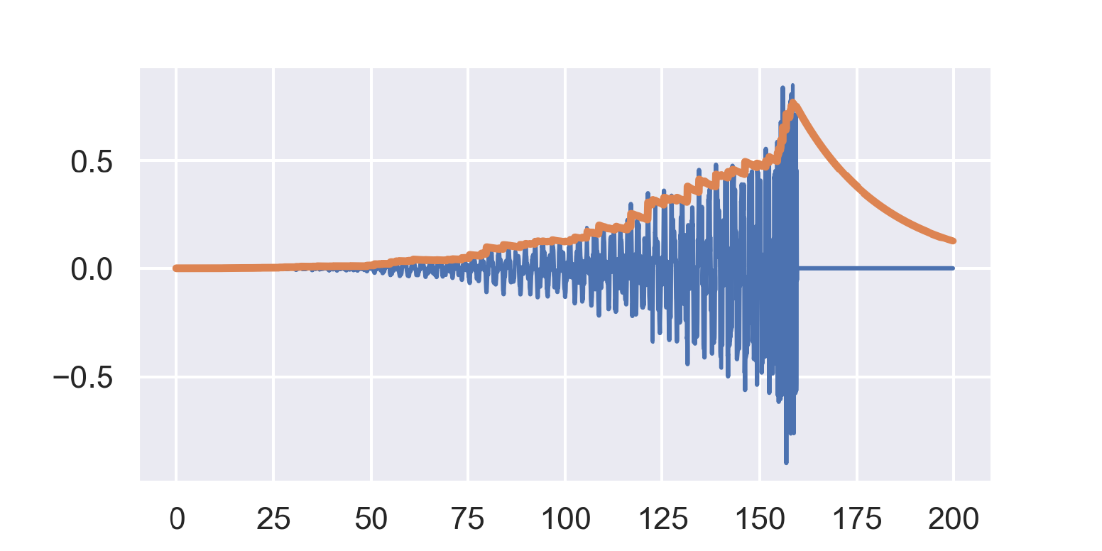
In this case, when the input value is higher than the previous output, we weight by a_. When the input value is lower, we weight by b_. This gives us a different response on the way up from on the way down. Generally you’d want to set a_ quite a bit lower than b_. For example, try a_ = 0.75 and b_ = 0.999:

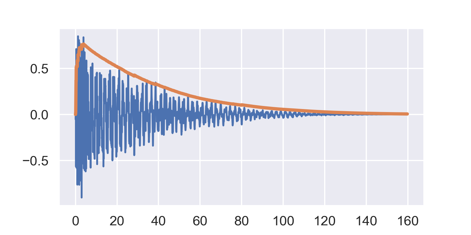
Out of all our followers, this one tracks the contour of the original sample the best. It looks the most like our hand-drawn contour above, and the sharp initial attack is more clearly separated from the long smooth decay. It’s important to note that the reason this particular follower works best is because the sound we’re tracking follows the fast attack / slow decay pattern.

As a counterexample, if we put the sample down, flip it and reverse it, the same follower doesn’t work so well any more:

It’s not a disaster exactly, but the envelope is too jagged on the way up, and extends too far past the end of the sample.

So this is not a magic follower that’s good for any sound in the world. It’s tuned for a specific class of sounds. Fortunately, this class includes lots of musical sounds: drums and percussion, plucked instuments, pianos, anything with a mallet, etc. In particular this kind of asymmetric follower is ideal for following the beat in music. The fast attack / slow decay follower is the main one I use in my projects.

How to set the decay parameters

Up until now, we’ve set the decay parameters a and b on a purely abstract scale. Can we express these values in terms of some real-world quantity?

The sample weighting follows an exponential decay according to the formula:

decay = a ^ num_samples

I like to think of exponential decay in terms of “half-lives.” The half-life is the number of samples that gives you a decay of 0.5:

0.5 = a ^ half_life_samples

Solving for a:

a = exp(log(0.5) / half_life_samples)

Of course, normally you probably think of things in terms of seconds or milliseconds instead of samples:

half_life_samples = (
    sample_rate *
    (half_life_millis / 1000.0)
)
a = exp(log(0.5) / half_life_samples)

With this formula, at a sample rate of 44100 Hz, and a 15 ms half-life, you’d get a decay parameter of about 0.999.

I typically start with an attack half-life somewhere around 1 ms, and a decay half-life in the neighborhood of 20 ms. Depending on the source material, sometimes I’ll dial the release up to as much as 100 ms.

What’s next?

In a future post, I’ll share some ideas about what you can do with the output of the envelope follower.